Closing the Gap: Telemetry vs Simulation

Progress update.

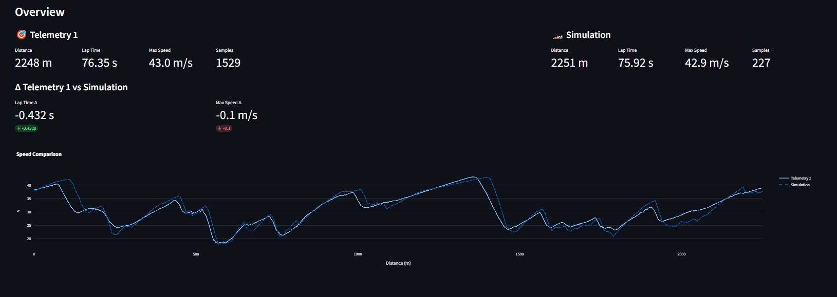
The latest build brings the simulation lap trace very close to real telemetry. Over most of the lap the velocity profiles lie nearly on top of each other. Remaining differences cluster at:

• Exit of low‑speed corners (torque application / tire longitudinal model)
• Peak speed regions (drag + powertrain efficiency blend)
• Brake zones (effective mu and weight transfer timing)

What’s driving the improved match?

Recent physics upgrades:

• Friction ellipse for combined tire grip (lateral + longitudinal)

Real tires can’t deliver maximum grip in both the lateral (cornering) and longitudinal (braking/acceleration) directions at the same time. The friction ellipse models this tradeoff, ensuring the total force stays within the tire’s physical limit. The combined grip is typically represented by:

(F_x / μF_z)² + (F_y / μF_z)² ≤ 1

Where:

• F_x = longitudinal force (acceleration/braking)
• F_y = lateral force (cornering)
• μ = effective friction coefficient (may be load-dependent, see below)
• F_z = normal load on the tire

This ensures that as you use more grip for braking or acceleration, less is available for cornering, and vice versa—matching real-world tire behavior.

• Non-linear tire grip (μ)

Tire grip is not a simple linear function of slip; instead, it follows a non-linear relationship that captures how tires generate peak force at moderate slip and then lose grip as slip increases further. This is often modeled using a simplified Pacejka “Magic Formula” or similar approach. However, for the current model, the effective friction coefficient is load-sensitive and computed as:

μ_eff = μ_nominal · (F_z / F_ref)^α

Where:

• μ_eff = effective friction coefficient
• μ_nominal = nominal (reference) friction coefficient
• F_z = normal load on the tire
• F_ref = reference load (for normalization)
• α = load sensitivity exponent (typically negative; grip decreases with load)

This non-linearity is critical for realistic simulation of tire behavior, especially near the limits of adhesion.

• Powertrain: improved gear ratio selection logic, linear interpolation of torque curve

• Rolling resistance

Rolling resistance opposes motion and is primarily due to tire deformation and internal friction. In the current model, it’s calculated as a sum of a constant term and a speed-dependent term:

F_rr = c₀ + c₁ · v

Where:

• F_rr = rolling resistance force
• c₀ = constant rolling resistance coefficient (depends on tire and surface)
• c₁ = speed-dependent coefficient
• v = vehicle speed

This approach captures both the baseline resistance and the increase with speed, improving accuracy over a purely constant model.

• Smoother distance integration: adaptive step size for high-curvature regions

Where we go next: systematic parameter fitting over multiple laps.

Core idea: treat the sim parameters as a vector p and minimize a cost J(p) across N laps of telemetry.

Candidate cost function:

J(p) = Σ_lap [ w_v · RMSE_v + w_a · RMSE_a + w_t · |Δt_lap| + w_evt · Σ_events RMSE_event-window ]

Process sketch, right out of the ML playbook:

1. Run simulation with current p;
2. Compute residual vector r; normalize each component.
3. Use bounded optimizer
4. Re-sim all laps in batch (vectorized per segment).
5. Iterate until ΔJ below tolerance or max iterations.

Safeguards:

• Regularization: penalize large deviations from baseline physical plausibility.
• Cross-validation: hold out one lap to detect overfitting.
• Parameter coupling: enforce aero drag ≤ physical engine force at top speed.

Once this pipeline is in place we shift from manual tweaking to data-driven convergence. That accelerates development and builds confidence before adding higher fidelity (transient tire stiffness, thermal effects, track elevation).

Next update: implementing the batch optimizer

Stay tuned.